40 how to change excel chart data labels to custom values

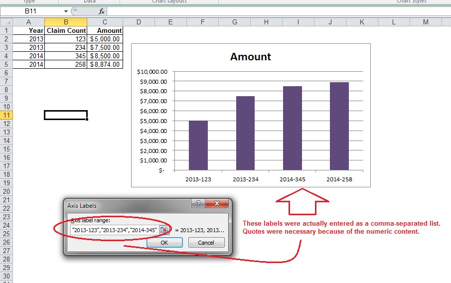
Changing range of data labels in chart - Excel Charting & Graphing ... Try-right click on chart to get context menu select 'Source Data...' click on the 'Series' tab at the bottom of the 'Series' tab there will be an range selection box labeled 'Category (X) axis labels' where you can select the range Custom Chart Data Labels In Excel With Formulas Follow the steps below to create the custom data labels. Select the chart label you want to change. In the formula-bar hit = (equals), select the cell reference containing your chart label's data. In this case, the first label is in cell E2. Finally, repeat for all your chart laebls.

Change the format of data labels in a chart Tip: To switch from custom text back to the pre-built data labels, click Reset Label Text under Label Options. To format data labels, select your chart, and then in the Chart Design tab, click Add Chart Element > Data Labels > More Data Label Options. Click Label Options and under Label Contains, pick the options you want.

How to change excel chart data labels to custom values

excel - Formatting chart data labels with VBA - Stack Overflow Here's the code so far: Sub FixLabels (whichchart As String) Dim cht As Chart Dim i, z As Variant Dim seriesname, seriesfmt As String Dim seriesrng As Range Set cht = Sheets ("Dashboard").ChartObjects (whichchart).Chart For i = 1 To cht.SeriesCollection.Count If cht.SeriesCollection (i).name = "#N/D" Then cht.SeriesCollection (i).DataLabels ... Apply Custom Data Labels to Charted Points - Peltier Tech Click once on a label to select the series of labels. Click again on a label to select just that specific label. Double click on the label to highlight the text of the label, or just click once to insert the cursor into the existing text. Type the text you want to display in the label, and press the Enter key. How to Customize Your Excel Pivot Chart Data Labels - dummies If you want to label data markers with a category name, select the Category Name check box. To label the data markers with the underlying value, select the Value check box. In Excel 2007 and Excel 2010, the Data Labels command appears on the Layout tab. Also, the More Data Labels Options command displays a dialog box rather than a pane.

How to change excel chart data labels to custom values. support.microsoft.com › en-us › officeAdd or remove data labels in a chart - support.microsoft.com When the Data Label Range dialog box appears, go back to the spreadsheet and select the range for which you want the cell values to display as data labels. When you do that, the selected range will appear in the Data Label Range dialog box. Then click OK. The cell values will now display as data labels in your chart. Is there a way to change the order of Data Labels? Please try to double click the the part of the label value, and choose the one you want to show to change the order. Thanks, Rena ----------------------- * Beware of scammers posting fake support numbers here. * Once complete conversation about this topic, kindly Mark and Vote any replies to benefit others reading this thread. Report abuse How to Use Cell Values for Excel Chart Labels Select the chart, choose the "Chart Elements" option, click the "Data Labels" arrow, and then "More Options." Uncheck the "Value" box and check the "Value From Cells" box. Select cells C2:C6 to use for the data label range and then click the "OK" button. The values from these cells are now used for the chart data labels. Custom Data Labels with Colors and Symbols in Excel Charts - [How To] To apply custom format on data labels inside charts via custom number formatting, the data labels must be based on values. You have several options like series name, value from cells, category name. But it has to be values otherwise colors won't appear. Symbols issue is quite beyond me.

› charts › percentage-changePercentage Change Chart - Automate Excel This tutorial will demonstrate how to create a Percentage Change Chart in all versions of Excel. Percentage Change – Free Template Download Download our free Percentage Template for Excel. Download Now Percentage Change Chart – Excel Starting with your Graph In this example, we’ll start with the graph that shows Revenue for the last 6… How to add or move data labels in Excel chart? - ExtendOffice 1. Click the chart to show the Chart Elements button . 2. Then click the Chart Elements, and check Data Labels, then you can click the arrow to choose an option about the data labels in the sub menu. See screenshot: Excel charts: how to move data labels to legend - Microsoft Tech Community You can't do that, but you can show a data table below the chart instead of data labels: Click anywhere on the chart. On the Design tab of the ribbon (under Chart Tools), in the Chart Layouts group, click Add Chart Element > Data Table > With Legend Keys (or No Legend Keys if you prefer) Excel Custom Data Labels with Symbols that change Colors ... - YouTube In this tutorial we will learn how to format Data labels in Excel Charts to make them dynamically change their colors. And also how to insert any symbols in ...

Use custom formats in an Excel chart's axis and data labels Right-click the Axis area and choose Format Axis from the context menu. If you don't see Format Axis, right-click another spot. Choose Number in the left pane. (In Excel 2003, click the Number ... Add / Move Data Labels in Charts - Excel & Google Sheets Check Data Labels . Change Position of Data Labels. Click on the arrow next to Data Labels to change the position of where the labels are in relation to the bar chart. Final Graph with Data Labels. After moving the data labels to the Center in this example, the graph is able to give more information about each of the X Axis Series. › excel › excel-chart-data-rangeModify Excel Chart Data Range | CustomGuide The new data needs to be in cells adjacent to the existing chart data. Rename a Data Series. Charts are not completely tied to the source data. You can change the name and values of a data series without changing the data in the worksheet. Select the chart; Click the Design tab. Click the Select Data button. Excel Custom Chart Labels - My Online Training Hub Step 1: Select cells A26:D38 and insert a column Chart. Step 2: Select the Max series and plot it on the Secondary Axis: double click the Max series > Format Data Series > Secondary Axis: Step 3: Insert labels on the Max series: right-click series > Add Data Labels: Step 4: Change the horizontal category axis for the Max series: right-click ...

Excel Chart Series Name Concatenate - chastity captions

Excel charts: add title, customize chart axis, legend and data labels ... Select the chart and go to the Chart Tools tabs ( Design and Format) on the Excel ribbon. Right-click the chart element you would like to customize, and choose the corresponding item from the context menu. Use the chart customization buttons that appear in the top right corner of your Excel graph when you click on it.

How to add labels to the mosaic plot - Microsoft Excel 365

Custom data labels in a chart - Get Digital Help Press with right mouse button on on any data series displayed in the chart. Press with mouse on "Add Data Labels". Press with mouse on Add Data Labels". Double press with left mouse button on any data label to expand the "Format Data Series" pane. Enable checkbox "Value from cells".

How to Change Date Formatting for Grouped Pivot Table Fields - Excel Campus

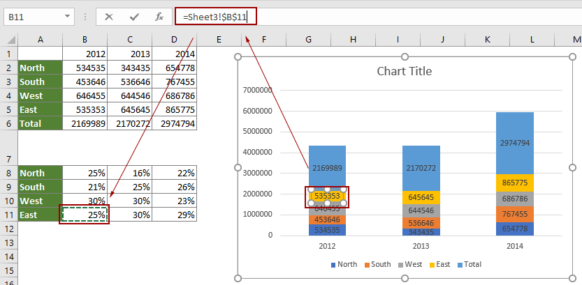
excel - How do I update the data label of a chart? - Stack Overflow Select the data label Then, place your cursor in Excel's Formula Bar, and enter the formula like ='Sheet2'!$C$3. Now, that data label is associated by the formula, to the cell C3, which contains the desired data label that we built above. Repeat as needed. Note: The sheet name is required in this formula.

Excel Bar Chart Percentage Label - Free Table Bar Chart

Make your Excel charts easier to read with custom data labels One way you can make your chart easier to read is to. remove the data series markers altogether and replace them with custom data. labels. For example, suppose you have the Months listed in A6:A17 ...

How To Change X Axis Labels In Excel

› excel-chart-verticalExcel Chart Vertical Axis Text Labels - My Online Training Hub To fix it: select the dummy series line in the chart > Right-click > Change Series Chart Type. Choose a Bar Chart. This will switch the dummy series to the secondary axis and you should have 3 axes displayed, but wait, you need more! The one axis we really want, the bar chart vertical axis, is missing:

34 Label Chart In Excel - Labels Database 2020

How to add data labels from different column in an Excel chart? Click any data label to select all data labels, and then click the specified data label to select it only in the chart. 3. Go to the formula bar, type =, select the corresponding cell in the different column, and press the Enter key. See screenshot: 4. Repeat the above 2 - 3 steps to add data labels from the different column for other data points.

How to Change Excel Chart Data Labels to Custom Values?

Excel Chart Data Labels-Modifying Orientation - Microsoft Community In reply to PaulaAB's post on September 13, 2016. Hi Paula, You can right click on the data label part then select Format Axis. Click on the Size & Properties tab then adjust the Text Direction or Custom Angle. Thanks,

32 How To Label Graphs In Excel - Labels Database 2020

How to Change Axis Values in Excel - Excelchat Right-click on the chart and choose Select Data Click on the button Switch Row/Column and press OK Figure 11. Switch x and y axis As a result, switches x and y axis and each store represent one series: Figure 12. How to swap x and y axis The chart will have more logic if we track store values per years.

Share :